Google Sheets Conditional Formatting Entire Row
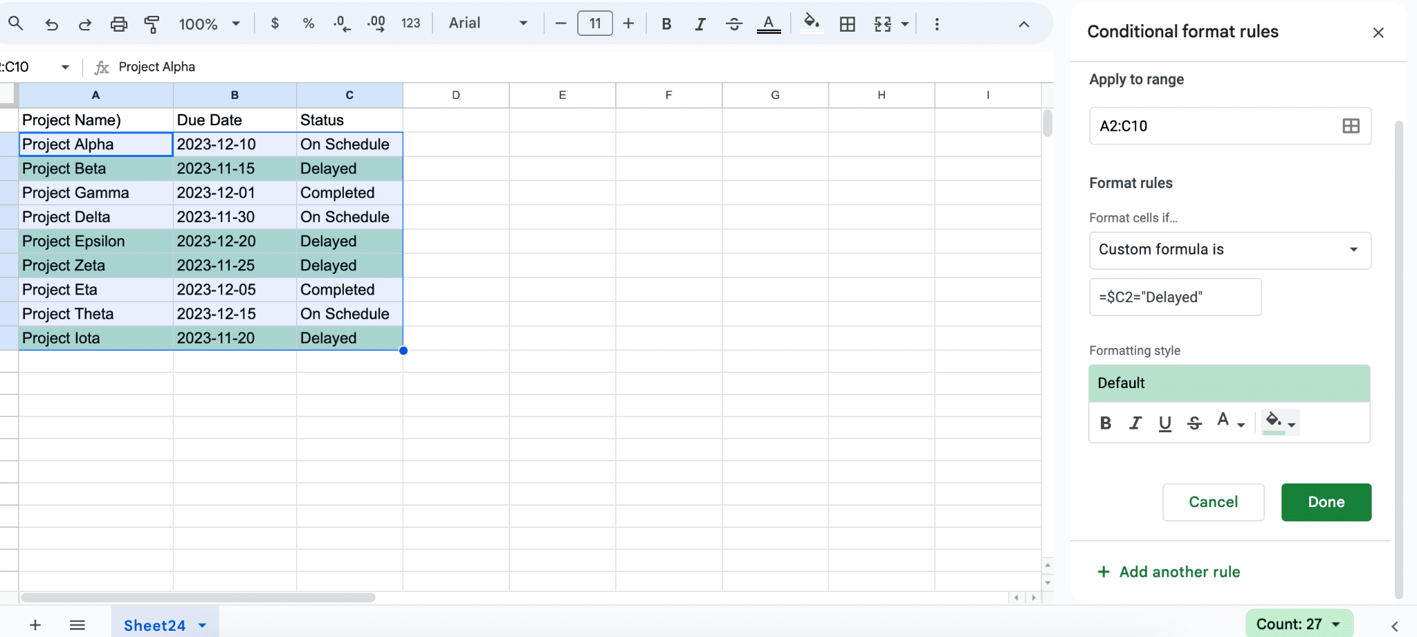
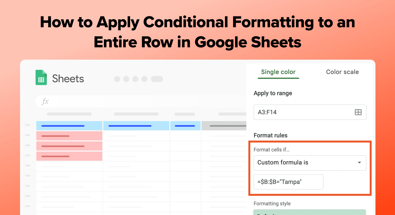
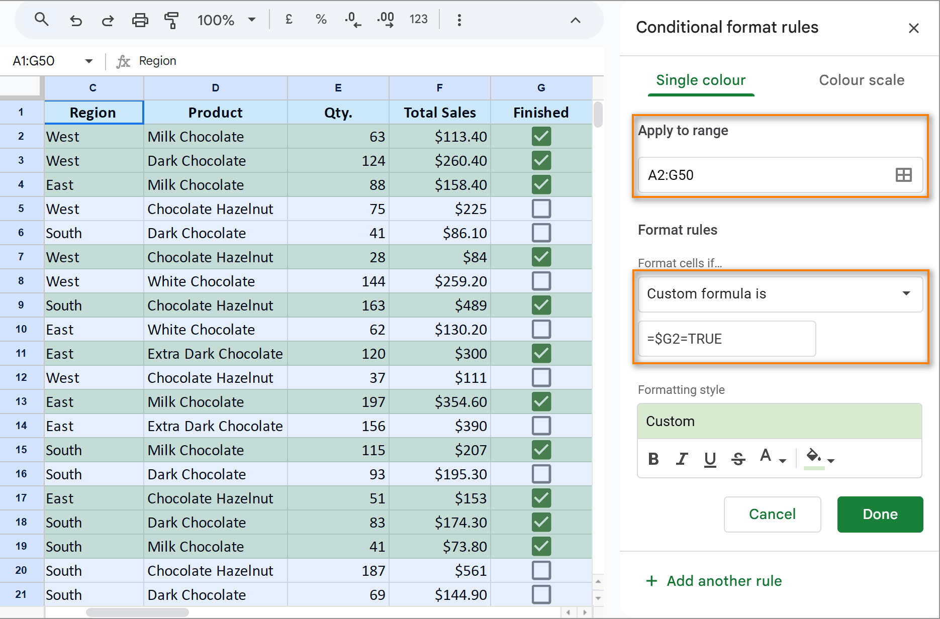
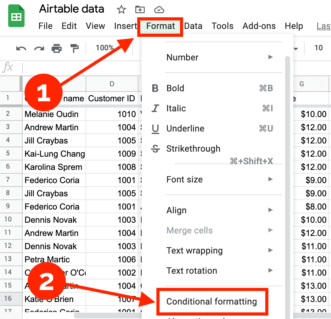
Google Sheets Conditional Formatting Entire Row - We’ll assume you have a dataset with sales figures, and you want. Let’s create a simple conditional formatting rule that applies to an entire row. For example, when the author in column c is 'colleen hoover,' we can change the background formatting for the entire row. To format an entire row based on the value of one of the cells in that row: The key principle in highlighting entire rows in google sheets is to employ absolute columns and relative rows. On your computer, open a spreadsheet in google sheets.
Let’s create a simple conditional formatting rule that applies to an entire row. To format an entire row based on the value of one of the cells in that row: We’ll assume you have a dataset with sales figures, and you want. For example, when the author in column c is 'colleen hoover,' we can change the background formatting for the entire row. The key principle in highlighting entire rows in google sheets is to employ absolute columns and relative rows. On your computer, open a spreadsheet in google sheets.
The key principle in highlighting entire rows in google sheets is to employ absolute columns and relative rows. For example, when the author in column c is 'colleen hoover,' we can change the background formatting for the entire row. Let’s create a simple conditional formatting rule that applies to an entire row. On your computer, open a spreadsheet in google sheets. To format an entire row based on the value of one of the cells in that row: We’ll assume you have a dataset with sales figures, and you want.

Apply Conditional Formatting To An Entire Row in Google Sheets
To format an entire row based on the value of one of the cells in that row: Let’s create a simple conditional formatting rule that applies to an entire row. For example, when the author in column c is 'colleen hoover,' we can change the background formatting for the entire row. On your computer, open a spreadsheet in google sheets..
Apply Conditional Formatting to Entire Rows in Google Sheets
The key principle in highlighting entire rows in google sheets is to employ absolute columns and relative rows. For example, when the author in column c is 'colleen hoover,' we can change the background formatting for the entire row. On your computer, open a spreadsheet in google sheets. We’ll assume you have a dataset with sales figures, and you want..

Apply Conditional Formatting To An Entire Row in Google Sheets
Let’s create a simple conditional formatting rule that applies to an entire row. For example, when the author in column c is 'colleen hoover,' we can change the background formatting for the entire row. The key principle in highlighting entire rows in google sheets is to employ absolute columns and relative rows. On your computer, open a spreadsheet in google.
Apply Conditional Formatting to Entire Rows in Google Sheets
We’ll assume you have a dataset with sales figures, and you want. The key principle in highlighting entire rows in google sheets is to employ absolute columns and relative rows. To format an entire row based on the value of one of the cells in that row: For example, when the author in column c is 'colleen hoover,' we can.

How To Apply Conditional Formatting Across An Entire Row In Google Sheets
On your computer, open a spreadsheet in google sheets. The key principle in highlighting entire rows in google sheets is to employ absolute columns and relative rows. We’ll assume you have a dataset with sales figures, and you want. To format an entire row based on the value of one of the cells in that row: For example, when the.

Google Sheets Conditional Formatting with Custom Formula Yagisanatode
On your computer, open a spreadsheet in google sheets. Let’s create a simple conditional formatting rule that applies to an entire row. We’ll assume you have a dataset with sales figures, and you want. For example, when the author in column c is 'colleen hoover,' we can change the background formatting for the entire row. The key principle in highlighting.
Apply Conditional Formatting To Entire Row In Google Sheets Medium
We’ll assume you have a dataset with sales figures, and you want. Let’s create a simple conditional formatting rule that applies to an entire row. To format an entire row based on the value of one of the cells in that row: For example, when the author in column c is 'colleen hoover,' we can change the background formatting for.
Complete guide to Google Sheets conditional formatting rules, formulas
To format an entire row based on the value of one of the cells in that row: The key principle in highlighting entire rows in google sheets is to employ absolute columns and relative rows. We’ll assume you have a dataset with sales figures, and you want. For example, when the author in column c is 'colleen hoover,' we can.
Conditional Formatting in Google Sheets Explained Coupler.io Blog
On your computer, open a spreadsheet in google sheets. The key principle in highlighting entire rows in google sheets is to employ absolute columns and relative rows. We’ll assume you have a dataset with sales figures, and you want. For example, when the author in column c is 'colleen hoover,' we can change the background formatting for the entire row..

Apply Conditional Formatting To An Entire Row in Google Sheets
For example, when the author in column c is 'colleen hoover,' we can change the background formatting for the entire row. To format an entire row based on the value of one of the cells in that row: We’ll assume you have a dataset with sales figures, and you want. The key principle in highlighting entire rows in google sheets.
The Key Principle In Highlighting Entire Rows In Google Sheets Is To Employ Absolute Columns And Relative Rows.
To format an entire row based on the value of one of the cells in that row: For example, when the author in column c is 'colleen hoover,' we can change the background formatting for the entire row. Let’s create a simple conditional formatting rule that applies to an entire row. On your computer, open a spreadsheet in google sheets.