Laplace Transform Sheet
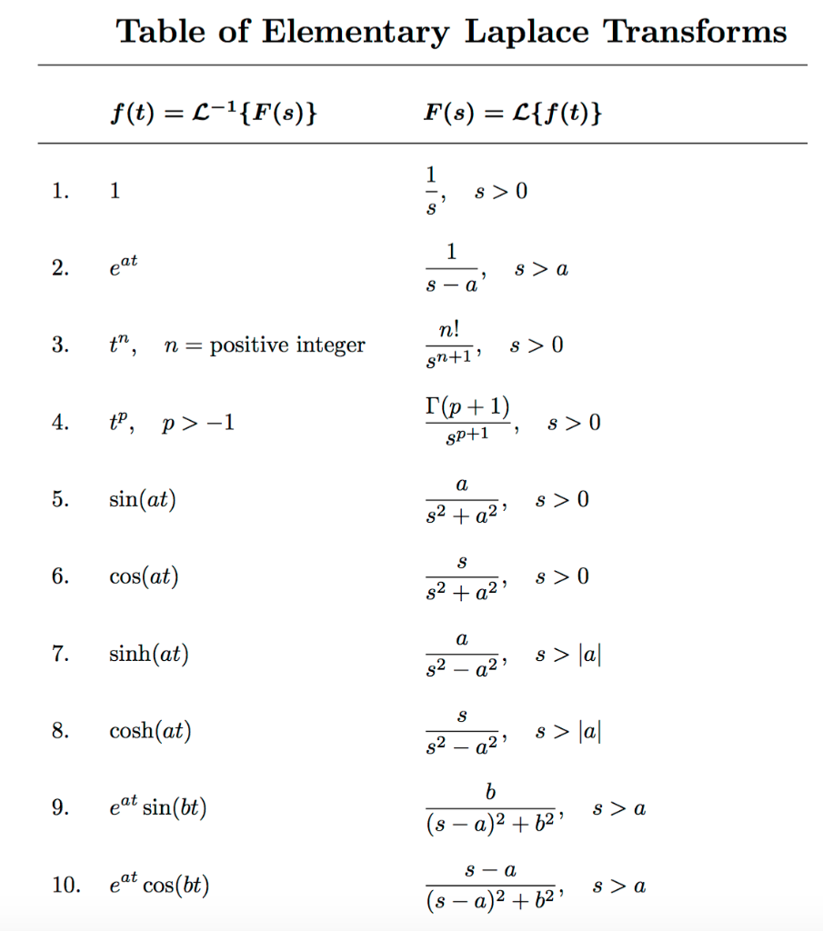
Laplace Transform Sheet - Table of laplace transforms f(t) l[f(t)] = f(s) 1 1 s (1) eatf(t) f(s a) (2) u(t a) e as s (3) f(t a)u(t a) e asf(s) (4) (t) 1 (5) (t stt 0) e 0 (6) tnf(t) ( 1)n dnf(s) dsn (7) f0(t) sf(s) f(0) (8) fn(t) snf(s) s(n 1)f(0). S2lfyg sy(0) y0(0) + 3slfyg. We give as wide a variety of laplace transforms as possible including some that aren’t often given. Laplace table, 18.031 2 function table function transform region of convergence 1 1=s re(s) >0 eat 1=(s a) re(s) >re(a) t 1=s2 re(s) >0 tn n!=sn+1 re(s) >0 cos(!t) s. In what cases of solving odes is the present method. (b) use rules and solve: This section is the table of laplace transforms that we’ll be using in the material. Solve y00+ 3y0 4y= 0 with y(0) = 0 and y0(0) = 6, using the laplace transform. State the laplace transforms of a few simple functions from memory. What are the steps of solving an ode by the laplace transform?
In what cases of solving odes is the present method. Laplace table, 18.031 2 function table function transform region of convergence 1 1=s re(s) >0 eat 1=(s a) re(s) >re(a) t 1=s2 re(s) >0 tn n!=sn+1 re(s) >0 cos(!t) s. (b) use rules and solve: What are the steps of solving an ode by the laplace transform? This section is the table of laplace transforms that we’ll be using in the material. State the laplace transforms of a few simple functions from memory. Solve y00+ 3y0 4y= 0 with y(0) = 0 and y0(0) = 6, using the laplace transform. We give as wide a variety of laplace transforms as possible including some that aren’t often given. Table of laplace transforms f(t) l[f(t)] = f(s) 1 1 s (1) eatf(t) f(s a) (2) u(t a) e as s (3) f(t a)u(t a) e asf(s) (4) (t) 1 (5) (t stt 0) e 0 (6) tnf(t) ( 1)n dnf(s) dsn (7) f0(t) sf(s) f(0) (8) fn(t) snf(s) s(n 1)f(0). S2lfyg sy(0) y0(0) + 3slfyg.
This section is the table of laplace transforms that we’ll be using in the material. S2lfyg sy(0) y0(0) + 3slfyg. State the laplace transforms of a few simple functions from memory. We give as wide a variety of laplace transforms as possible including some that aren’t often given. What are the steps of solving an ode by the laplace transform? Laplace table, 18.031 2 function table function transform region of convergence 1 1=s re(s) >0 eat 1=(s a) re(s) >re(a) t 1=s2 re(s) >0 tn n!=sn+1 re(s) >0 cos(!t) s. In what cases of solving odes is the present method. Table of laplace transforms f(t) l[f(t)] = f(s) 1 1 s (1) eatf(t) f(s a) (2) u(t a) e as s (3) f(t a)u(t a) e asf(s) (4) (t) 1 (5) (t stt 0) e 0 (6) tnf(t) ( 1)n dnf(s) dsn (7) f0(t) sf(s) f(0) (8) fn(t) snf(s) s(n 1)f(0). Solve y00+ 3y0 4y= 0 with y(0) = 0 and y0(0) = 6, using the laplace transform. (b) use rules and solve:
Sheet 1. The Laplace Transform
We give as wide a variety of laplace transforms as possible including some that aren’t often given. In what cases of solving odes is the present method. (b) use rules and solve: This section is the table of laplace transforms that we’ll be using in the material. What are the steps of solving an ode by the laplace transform?

Laplace Transform Full Formula Sheet
Laplace table, 18.031 2 function table function transform region of convergence 1 1=s re(s) >0 eat 1=(s a) re(s) >re(a) t 1=s2 re(s) >0 tn n!=sn+1 re(s) >0 cos(!t) s. This section is the table of laplace transforms that we’ll be using in the material. We give as wide a variety of laplace transforms as possible including some that aren’t.
Laplace Transforms Formula Sheet Table Of Laplace Transforms F T L
In what cases of solving odes is the present method. We give as wide a variety of laplace transforms as possible including some that aren’t often given. This section is the table of laplace transforms that we’ll be using in the material. State the laplace transforms of a few simple functions from memory. What are the steps of solving an.
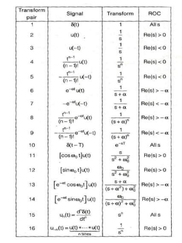
Table Laplace Transform PDF PDF
In what cases of solving odes is the present method. Laplace table, 18.031 2 function table function transform region of convergence 1 1=s re(s) >0 eat 1=(s a) re(s) >re(a) t 1=s2 re(s) >0 tn n!=sn+1 re(s) >0 cos(!t) s. This section is the table of laplace transforms that we’ll be using in the material. Table of laplace transforms f(t).

Laplace Transform Table
We give as wide a variety of laplace transforms as possible including some that aren’t often given. Solve y00+ 3y0 4y= 0 with y(0) = 0 and y0(0) = 6, using the laplace transform. What are the steps of solving an ode by the laplace transform? Table of laplace transforms f(t) l[f(t)] = f(s) 1 1 s (1) eatf(t) f(s.

Inverse Laplace Transform Table LandenrilMoon
Solve y00+ 3y0 4y= 0 with y(0) = 0 and y0(0) = 6, using the laplace transform. Laplace table, 18.031 2 function table function transform region of convergence 1 1=s re(s) >0 eat 1=(s a) re(s) >re(a) t 1=s2 re(s) >0 tn n!=sn+1 re(s) >0 cos(!t) s. We give as wide a variety of laplace transforms as possible including some.

Laplace Transform Formula Sheet PDF
Solve y00+ 3y0 4y= 0 with y(0) = 0 and y0(0) = 6, using the laplace transform. What are the steps of solving an ode by the laplace transform? Table of laplace transforms f(t) l[f(t)] = f(s) 1 1 s (1) eatf(t) f(s a) (2) u(t a) e as s (3) f(t a)u(t a) e asf(s) (4) (t) 1 (5).

Table of Laplace Transforms Hyperbolic Geometry Theoretical Physics
We give as wide a variety of laplace transforms as possible including some that aren’t often given. Laplace table, 18.031 2 function table function transform region of convergence 1 1=s re(s) >0 eat 1=(s a) re(s) >re(a) t 1=s2 re(s) >0 tn n!=sn+1 re(s) >0 cos(!t) s. State the laplace transforms of a few simple functions from memory. (b) use.

Laplace Transform Sheet PDF
State the laplace transforms of a few simple functions from memory. S2lfyg sy(0) y0(0) + 3slfyg. Table of laplace transforms f(t) l[f(t)] = f(s) 1 1 s (1) eatf(t) f(s a) (2) u(t a) e as s (3) f(t a)u(t a) e asf(s) (4) (t) 1 (5) (t stt 0) e 0 (6) tnf(t) ( 1)n dnf(s) dsn (7) f0(t).
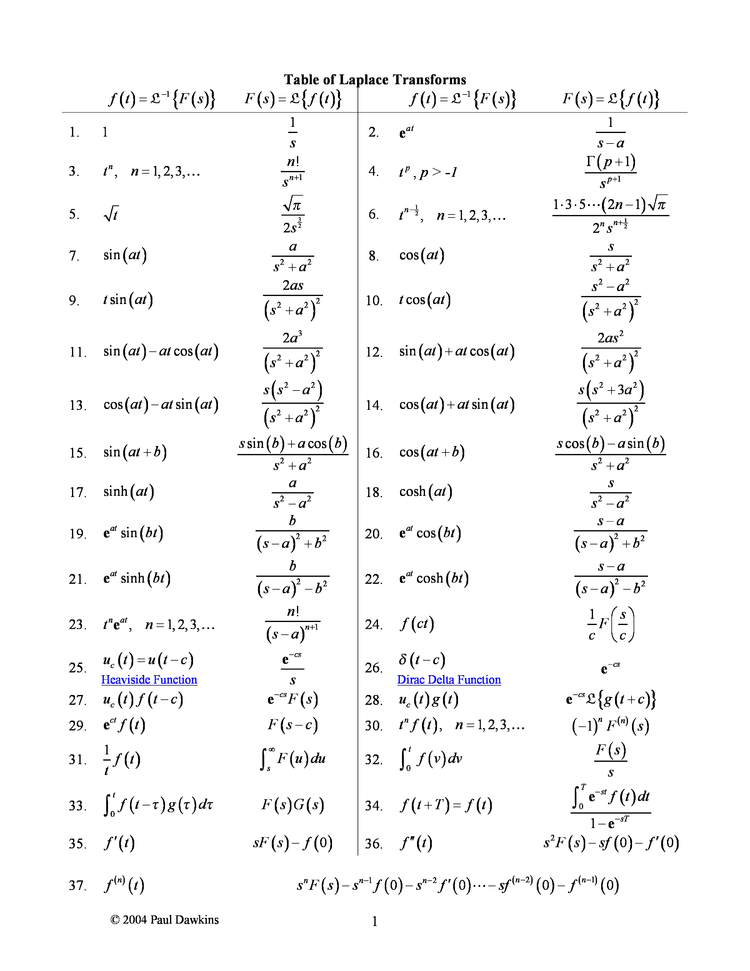
Table of Laplace Transforms Cheat Sheet by Cheatography Download free
What are the steps of solving an ode by the laplace transform? (b) use rules and solve: Solve y00+ 3y0 4y= 0 with y(0) = 0 and y0(0) = 6, using the laplace transform. Table of laplace transforms f(t) l[f(t)] = f(s) 1 1 s (1) eatf(t) f(s a) (2) u(t a) e as s (3) f(t a)u(t a) e.
Solve Y00+ 3Y0 4Y= 0 With Y(0) = 0 And Y0(0) = 6, Using The Laplace Transform.
In what cases of solving odes is the present method. This section is the table of laplace transforms that we’ll be using in the material. Table of laplace transforms f(t) l[f(t)] = f(s) 1 1 s (1) eatf(t) f(s a) (2) u(t a) e as s (3) f(t a)u(t a) e asf(s) (4) (t) 1 (5) (t stt 0) e 0 (6) tnf(t) ( 1)n dnf(s) dsn (7) f0(t) sf(s) f(0) (8) fn(t) snf(s) s(n 1)f(0). State the laplace transforms of a few simple functions from memory.
(B) Use Rules And Solve:
We give as wide a variety of laplace transforms as possible including some that aren’t often given. S2lfyg sy(0) y0(0) + 3slfyg. Laplace table, 18.031 2 function table function transform region of convergence 1 1=s re(s) >0 eat 1=(s a) re(s) >re(a) t 1=s2 re(s) >0 tn n!=sn+1 re(s) >0 cos(!t) s. What are the steps of solving an ode by the laplace transform?